How was it made?
Ultraviolet spectra simulator for proteins and DNA

Data sources

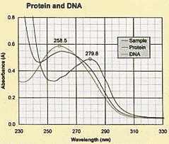
Experimental spectra of protein and DNA.

The source material was the image file from:

• Spectrophotometric Bio Analysis (GENEQ inc.)
  • http://www.geneq.com/catalog/en/sba.html
    Applications example:
    

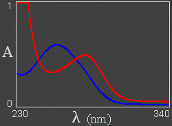
Curves were manually generated that would fit visually well to the two experimental curves. For this, we used User-Defined-Transforms in SigmaPlot where equations were combined from the SigmaPlot library (Graph > Plot Equation > Library > Peak )

• Lorentzian, 4 Parameter: y0+a/(1+((x-x0)/b)^2)
• Gaussian, 3 Parameter: a*exp(-.5*((x-x0)/b)^2)

(X,Y) data were generated in SigmaPlot every 2 nm. Combining one Lorentzian (for the baseline) and two Gaussians we achived reasonable superimposition with experimental spectra.

• col(1) = data(230,340,2)
• x=col(1)
  parm=4
  y0=cell(parm,2)/1000
• a=cell(parm,3)/1000
  x0=cell(parm,4)
  b=cell(parm,5)
• 1=cell(parm,8)/1000
  x01=cell(parm,9)
  b1=cell(parm,10)
• 2=cell(parm,13)/1000
  x02=cell(parm,14)
  b2=cell(parm,15)
• y=y0+a*exp(-.5*((x-x0)/b)^2)+a1*exp(-.5*((x-x01)/b1)^2)+a2/(1+((x-x02)/b2)^2)
  put y into col(parm+1)

Proteins:

y = 0.032 + 0.395 * exp(-0.5*((x-281)/11)^2)
              + 0.125 * exp(-0.5*((x-262)/9)^2)
              + 3.5 / (1+((x-228)/6.2)^2)

DNA:

y = 0.066 + 0.480 * exp(-0.5*((x-258)/13.5)^2)
              + 0.158 * exp(-0.5*((x-279)/10)^2)
              + 6.2 / (1+((x-200)/6.2)^2)

DNA gave A₂₆₀/A₂₈₀ = 1.63; this was changed to y = 0 + 0.505 * etc. to achieve a 1.8 ratio,
and for proteins too to y = 0 + etc.

With those, a function could be created that generates the combined spectra.

Implementation in a web page:

By following a similar development to what was used for circular dichroism spectra, Walter Zorn's JavaScript graphic library was used to achieve the drawing of the graph.

• http://www.walterzorn.com/jsgraphics/jsgraphics_e.htm

Data used to build the graphs are:

• the formulas adjusted to fit the simulated spectra are used in a JavaScript function that calculates Y values (screen pixels) for each X (screen pixels);
• to generate any combination for a sample, a linear combination of both functions is used, weighted according to the fraction of each kind of molecule.

Angel Herráez. Part of the Biomodel.uah.es website